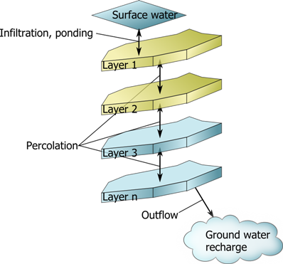
A one dimensional highly detailed model, comparable to models like BROOK90 (Federer 1995; Allen et al., 1998) or Hydrus 1D (Simunek et al., 2005), is developed through the allocation of a number of soil water storages, with connections based upon a Richards equation-based flux connector. This very short and simple example shows just the percolation through a homogeneous medium without any boundary flow. A more complete example with rainfall and graphical output can be found in the download section.

Create a project and one 1000m² cell

import cmf
from datetime import datetime,timedelta
project = cmf.project()
# Add one cell at position (0,0,0), Area=1000m2 with a surface water storage
cell = project.NewCell(x=0,y=0,z=0,area=1000, with_surfacewater=True)

Create a retention curve

r_curve = cmf.VanGenuchtenMualem(Ksat=1,phi=0.5,alpha=0.01,n=2.0)

Add ten layers of 10cm thickness

for i in range(10):
    depth = (i+1) * 0.1
    cell.add_layer(depth,r_curve)

Connect layers with Richards perc.

for upper,lower in zip(cell.layers[:-1],cell.layers[1:]):

cmf.Richards(upper,lower)

this can be shorten as

cell.install_connection(cmf.Richards)

Using this command, all layers of the cell get connected with Richards equation.

Now we need to create an integrator for the resulting system. Since the Richards equation procduces a very stiff (difficult to solve) system, one needs to use an implicit solver with an adaptive time stepping scheme. The CVodeKrylov, a wrapper for the CVODE-solver by Hindmarsh et al. (2005) is such a solver and recommended for all cmf models using Richards equation.

solver = cmf.CVodeKrylov(project,1e-6)

solver.t = cmf.Time(1,1,2011)

Now we set the initial conditions

# Set all layers to a potential of -2 m
cell.saturated_depth = 2.
# 100 mm water in the surface water storage for percolation
cell.surfacewater.depth = 0.1

This is the setup code for our simple 1D Richards-Model. To run the model we create the run time loop using the solver.run iterator and we save soil moisture and potential for each layer into lists.

# Save potential and soil moisture for each layer,
# start with initial conditions
potential = [cell.layers.potential]
moisture = [cell.layers.theta]
# The run time loop, run for 7 days
for t in solver.run(solver.t,
                    solver.t + timedelta(days=7),
                    timedelta(hours=1)):
    potential.append(cell.layers.potential)
    moisture.append(cell.layers.theta)
    
# Plot results
from pylab import *
subplot(211)
plot(moisture)
ylabel(r'Soil moisture $\theta [m^3/m^3]$')
xlabel(r'$time [h]$')
grid()
subplot(212)
plot(potential)
ylabel(r'Water head $\Psi_{tot} [m]$')
xlabel(r'$time [h]$')
grid()

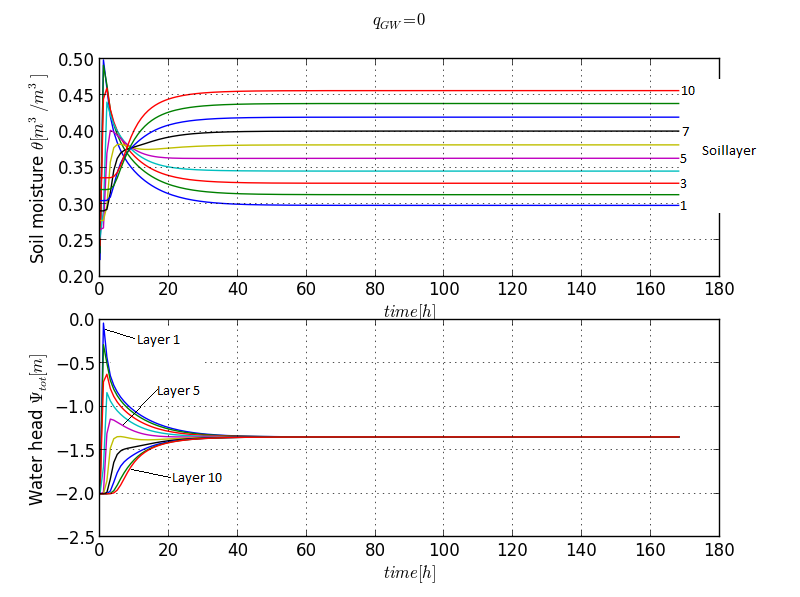
The upper graph shows the soil moisture content of each layer, the lower the water potential for each layer. The water table rises and a new hydrostatic equilibrium at 1.35 m below ground is established

Adding a groundwater boundary condition

As the next step, a fixed groundwater table as a lower boundary condition is introduced into our model. The following line needs to be inserted into the setup part of the script, eg. before setting the initial conditions:

# Create the boundary condition
gw = project.NewOutlet('groundwater',x=0,y=0,z=-2)
# Set the potential
gw.potential = -2 
# Connect the lowest layer to the groundwater using Richards percolation
gw_flux=cmf.Richards(cell.layers[-1],gw)

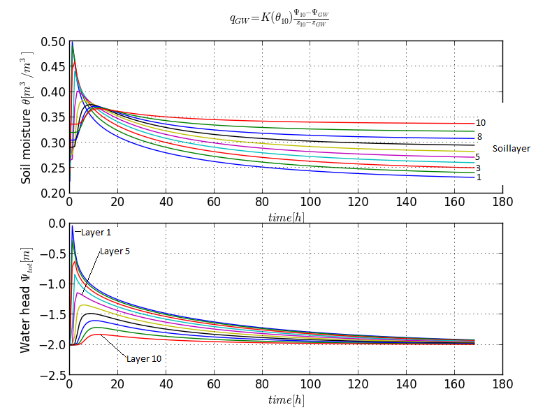
In this experiment, the water percolates through the soil and out of our model boundaries. The water content is at the end of the simulation period near to the orginal values.

Adding a groundwater boundary condition

Some links to the API help of objects used in this tutorial