In this chapter we will bring our 1D cell from [[wiki:CmfTut1d]|and the lateral connections from CmfTutDarcianLateralFlow and CmfTutSurfaceRunoff together to a complete hillslope model. As in these tutorials will not include rainfall and ET to keep the code better readable. With the information from CmfTutTestData, CmfTutMeteostation and [wiki:CmfTutET]] it should be possible to extend this tutorial on your own to a complete model.

Define the hillslope

Here we will define the catena of cells on the hillslope. For "real" applications, you will load the topography of the hill slope from a file

here we use a simple function z(x). The cmf project will be p again.

Import libraries, create project

import cmf
import numpy as np
def z(x): 
    return 10/(1+np.exp((x-100)/30))
# create a project
p = cmf.project()

Creating 20 cells

Our hill slope should have an exponential slope, is 200 m long and is discretized into 20 cells. By using different cell areas, a quasi-3D effect for converging or diverging fluxes could be applied, but in our example the area of each cell is fixed to 10m x 10m.

for i in range(20):
    x = i * 10.
    # create a cell with surface storage
    c = p.NewCell(x,0,z(x),100,True)

The topological connection of the cells is simple, we only need to connect each cell with its lower neighbor. The width of the connection is 10m.

for c_upper,c_lower in zip(p[:-1],p[1:]):

c_upper.topology.AddNeighbor(c_lower,10.)

Now, each cell needs to have soil layers, exactly the same way as in the setup code in [wiki:CmfTut1d], just with some other layer depth and the "default" Van Genuchten-Mualem retention curve - it is better to parameterize your soil type of course (Hydraulic head (subsurface)).

# Customize cells
for c in p:
    # create layers    
    for d in [0.02,0.05,0.1,0.2,0.3,0.5,0.75,1.0,1.25,1.5,1.75,2.]:
        rc = cmf.VanGenuchtenMualem(Ksat=50*np.exp(-d),alpha=0.1,n=2.0,phi=0.5)
        rc.w0 = 0.9996
        c.add_layer(d,rc)
    # set initial conditions
    c.saturated_depth=2.
    # use Richards connection
    c.install_connection(cmf.Richards)
    c.install_connection(cmf.GreenAmptInfiltration)
    # Add more connections here... (eg. ET, snowmelt, canopy overflow)

Using Darcy and KinematicSurfaceRunoff as lateral connections as in CmfTutDarcianLateralFlow and CmfTutSurfaceRunoff. Due to the defined topology, we can use the cmf.connect_cells_with_flux function.

cmf.connect_cells_with_flux(p,cmf.Darcy)

cmf.connect_cells_with_flux(p,cmf.KinematicSurfaceRunoff)

cmf.connect_cells_with_flux

connect_cells_with_flux(cells, connection, start_at_layer=0)

Definition __init__.py:30

Create boundary conditions and solver

Boundary conditions

For our example we will use the following boundary conditions:

1. No flow to the deep groundwater (impervious bedrock) 2. No flow at the upper side of the hillslope (upper side is water shed) 3. Steady rainfall of 10mm/day to each cell 4. Constant head boundary at the low end of the hillslope at 0.47m below the lowest cell in 10 m distance.

Boundary conditions 1 & 2 are implemented by doing nothing (no connection is no flow). Boundary condition 3 is applied as follows:

for c in p:

c.set_rainfall(10.)

Boundary condition 4 (outlet) is applied by using a DirichletBoundary, using the NewOutlet method of the project. The outlet is connected with the Darcy connection to each soil layer. The surface water of the lowest cell p\[\[-1\]|is connected to the outlet with KinematicSurfaceRunoff

outlet = p.NewOutlet('outlet',200,0,0)
for l in p[-1].layers:
    # create a Darcy connection with 10m flow width between each soil layer
    # and the outlet
    cmf.Darcy(l,outlet,FlowWidth=10.)
cmf.KinematicSurfaceRunoff(p[-1].surfacewater,outlet,10.)

Solver

The last thing needed for the complete setup code is the solver. With Richards and Darcy equation, we have again a stiff system and thus use the CVODE solver:

solver = cmf.CVodeKrylov(p,1e-9)

solver.t = datetime.datetime(2012,1,1)

Visualization and runtime loop

In the runtime code, you need to define which data should be collected during runtime and handle the data accordingly. In [wiki:CmfTut1d] we have used two different approaches - save data to a file during runtime and collect the data in a list for later visualization. You can of course apply both techniques here also. However, if you want to observe the state changes in a 2D hillslope and not only the runoff, an image with time on the one axis and depth on the other is not sufficient. Hence we are going to present the results live during the model run in an animation.

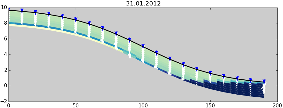
First we need a kind of drawing, that shows all states. As always in cmf, you can design the output as you like. One possibility, drawing everey layer as a sheared rectangle colored by a state variable and arrows indicating the flux between the layers is already bundled with cmf in the cmf.draw module - the hill_plot class. This class is not very well documented, but you can have a look to the source code.

This creates a hill_plot of our hillslope:

# Import the hill_plot
from cmf.draw import hill_plot
# Import some matplotlib stuff
from matplotlib.pylab import figure,show,cm
 
# Create a new matplotlib figure fig
fig = figure(figsize=(16,9))
# Create a subplot with a light grey background
ax = fig.add_subplot(111,axisbg='0.8')
# Create the hillplot for water filled pore space with using a yellow to green to blue colormap
image = hill_plot(p,solver.t,cmap=cm.YlGnBu)
# Set the scale for the arrows. This value will change from model to model.
image.scale = 100.
# white arrows are nicer to see
image.q_sub.set_facecolor('w')

Animations can be created using the FuncAnimation class from the matplotlib.animation module. The drawing (and in our case advancing of the model) is done in a function taking the frame number as the first argument:

def run(frame):
    # Run model for one day
    t = solver(cmf.day)
    # Update image
    image(t)

Last part is to create the animation object and show what we have done. The animation starts directly.

from matplotlib.animation import FuncAnimation
animation = FuncAnimation(fig,run,repeat=False,
                          frames=365)
show()

The result after 30 days of simulation looks like this:

Excercises

1. Stop the rain after 100days. (a few minutes) 2. Save the outlet water balance in a list and plot it after calculation (a few minutes) 3. Use real weather data (some more work) 4. Use ET, snowmelt etc. (a few minutes) 5. Go in the field, measure pF curves, collect meteo data and discharge and make a real model. Learn from model failure (time...)