Depending on your model design, you might need to use rather abstract concepts can help to realize your model - but not every model needs these connections.

The class names of these connections are not very good and will be changed in CMF 2.0. Starting with cmf 1.4 the new names are already available

Balancing water flux at one node

What does it mean?

The WaterbalanceFlux is a connection to route the water balance of a node somewhere else. The connection checks the flux over all other connections of the left node and routes any surplus to the right node, or in case of a negative water balance of the left node, additional water is fetched from the right node. Or as a mathematical expression:

\[ q_{N} = -\sum_{i=1}^{N-1} q_{j}(V, V_{j}) \]

The water balance connection levels always all other fluxes out: The sum of all fluxes (including the water balance connection) is zero.

\[ \sum_{i=1}^{N} q_{j}(V, V_{j}) = \frac{dV}{dt} = 0 \]

Hence, there is often no need anymore to leave the left node a storage, since no state change can happen there due to the water balance connection. You should therefore consider to change your storage into a "non-storing" node, like a boundary condition. If your water balance connection connects to the surface of a cell, you can (in most cases) create the cell without surface water storage

When do I want a water balance connection

In practice, we found mainly two situations, when to use the water balance connection:

at the cell surface
to connect submodels

However, a water balance connection might solve a problem for a totally new application of cmf, which we as the developers have not forseen. Be creative!

At the cell surface

When the user creates the first subsurface storage for a conceptual model with no surface water storage, this first layer is automatically connected with the surface via a water balance connection.

p = cmf.project()
# Create cell without surface water storage
c = p.NewCell(0, 0, 0, 1000, with_surfacewater=False)
l = c.add_layer(1.0)  # Add layer with 1000 mm capacity
print(cmf.describe(c.surfacewater))

results in:

{Surface water of cell #0}:
- waterbalance connection({Surface water of cell #0}<->{Layer #0 of cell #0})
- Rainfall({Constant rainfall of 0 mm/day}<->{Surface water of cell #0})

With this automatic construction, the mass balance of the system is ensured - no water can vanish at the surface node, which happens when the water balance of c.surfacewater.waterbalance(t) != 0.

If you choose to use an infiltration method that limits infiltration by saturation excess or hortonian overflow (e.g. ConceptualInfiltration), and the cell surface is still no storage, the local mass balance on the surface is not necessary zero, and the excess gets lost. To route the surface water excess without time lag to a river or the catchment outlet (good approximation for time steps > 1h), you can use the water balance connection again.

The following code is meant to expand the code snippet from above:

cmf.ConceptualInfiltration(l, c.surfacewater)
# Create outlet
out = p.NewOutlet('outlet')
# moves all infiltration excess to the outlet
cmf.WaterbalanceFlux(c.surfacewater, out)
print(cmf.describe(c.surfacewater))

results in:

{Surface water of cell #0}:
- waterbalance connection({Surface water of cell #0}<->{outlet})
- simple infiltration({Surface water of cell #0}<->{Layer #0 of cell #0})
- Rainfall({Constant rainfall of 0 mm/day}<->{Surface water of cell #0})

As a bridge between submodels

If the second example for the surface does not point to an outlet but another part of the model setup, eg. a river, the water balance connection is the bridge between the local (cell) sub model and the distributing river network. You can also place a collection node between the submodels for simplified observation of fluxes between these different model domains.

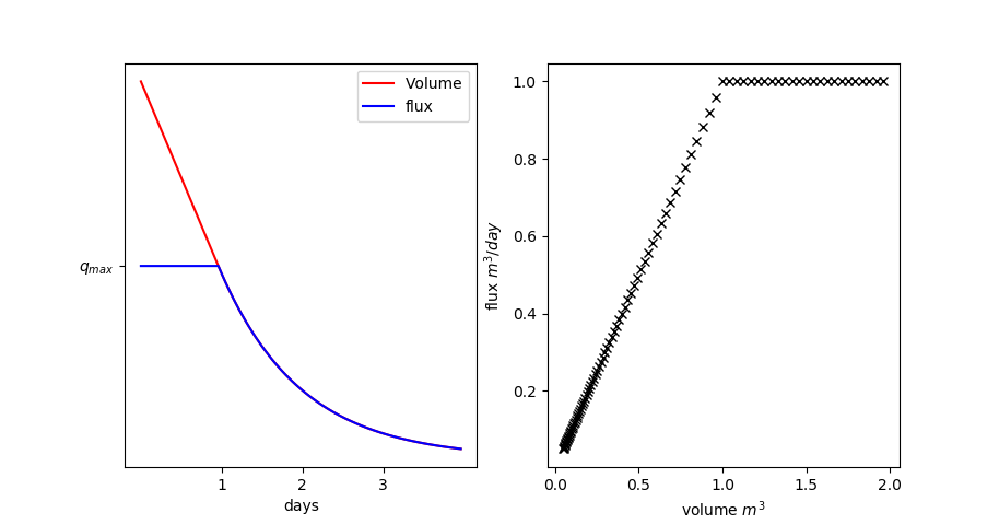
Keeping a flux constant as long as water is available

For some processes a constant flux from one water storage to another or a boundary condition is needed. These constant (but externally changeable) fluxes can be anthropogenic water fluxes, like the regulation of a dam or a pump rate, or some other process that has a flux limit. Eg. the model HBVlight assumes a constant percolation from the 1st to the 2nd groundwater storage. However, when the source becomes empty, the flux stops. To avoid a hard stop, the fluxes decreases linear to zero, when only volume for decrease time is left in the source storage.

Currently, this type of connection is called ConstantFlux.

p = cmf.project()
w = p.NewStorage('source')
o = p.NewOutlet('out')
import pylab as plt
# Add a constant flux
constflux = cmf.ConstantFlux(w, o, 1.0, flux_decrease_time=cmf.day)
w.volume = 2.0
solver = cmf.RKFIntegrator(p)
vol, flux = zip(*[(w.volume, w.flux_to(o, t)) 
                  for t in solver.run(cmf.Time(), cmf.day * 4, cmf.h)])
plt.subplot(1, 2, 1)
plt.plot(vol,color='r', label='Volume')
plt.plot(flux,color='b', label='flux')
plt.yticks([1], ['$q_{max}$'])
plt.xticks([24, 48, 72],[1, 2, 3])
plt.xlabel('days')
plt.legend()
plt.subplot(1, 2, 2)
plt.plot(vol, flux, 'kx')
plt.ylabel('flux $m^3/day$')
plt.xlabel('volume $m^3$') 

Keeping a state constant as long as water is available

This connection holds the state of a water storage constant getting or releasing water to the other node of the connection. The flux between the nodes is proportional to the difference between the state of the storage and the defined target state of the storage. This connection is called ConstantStateFlux.

Partitioning of a water flux calculated by another connection

PartitionFluxRoute reads the flux between two nodes (source and target1) and routes a fraction of the actual flux to a third node (target2) immediately and without a time lag. The PartitioningFluxRoute connects target1 with target2 but gets the flux from the other connection.

This can be used for divides in the network, bypassing layers as in BROOK90 or leaky connections in conceptual models. Another option is to divide a water flux into a fast and slow path way.