|
2.0.0b10
catchment modelling framework
|
|
2.0.0b10
catchment modelling framework
|
... is the title of a paper by Singh (2002), where he lists numerous examples from all scales of hydrology where a kinematic wave function has been found to be a valid descriptor for hydrological processes. Anyway, numerous more or less conceptional models in hydrology use kinematic wave like formulations to calculate fluxes. While some authors are happy to call every 1st order flux calculation using some exponent a kinematic wave, other authors like to see the term reserved for more "wave like" phenomens in hydrology.
Hence a number of different names exist for the same concept:
A generalized form for some approaches is:
\[ q(V) = Q_0 \cdot \theta^\beta\ (1) \]
where:
For cmf, using the finite volume approach, we need a consistent function to relate the stored water volume \(V\) in a water storage to the variable \(\theta\). So we define:
\[ \theta = \frac{V - V_{res}}{V_0}\ (2) \]
where:
The famous linear storage equation can be seen as a special case of this approach where \(\beta=1\). In that case, we can rearrange the formula above to:
\[ q(V) = \frac{Q_0}{V_0} \cdot (V-V_{res})\ (3) \]
Here the quotient \(\frac{Q_0}{V_0}\) becomes the inverse of the storage residence time \(t_r^{-1}\), which simplifies (3) to
\[ q(V) = \frac 1 {t_r [days]} \cdot (V-V_{res})\ (4) \]
for the linear case
Due to the different meanings of parameters between the linear and non-linear case, cmf provides now 2 distinct connections for the linear and the non-linear case.
The linear storage connection LinearStorageConnection implements (4) and takes the residence time in days and a residual water content in m³ as parameters. While the residence time must be given, the residual water content can be omitted and set to 0. Depending on system size and structure, residence times between minutes for surface water storages or fast drainages up to hundreds of years for large aquifers are suitable values.
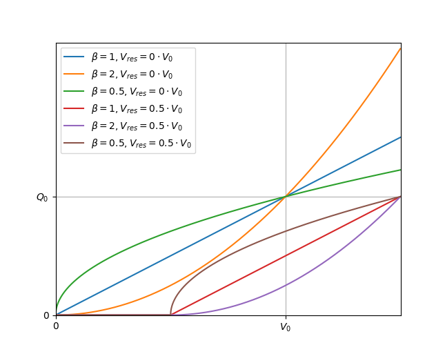
The power law connection (PowerLawConnection) needs the parameters Q0, V0 and beta as given in the generalized form of the power law equation. The reference flow \(Q_0 [\frac{m^3}{days}]\) occurs when the source water storage contains the reference volume \(V_0\) as mobile water. The curve shape parameter \(\beta\) bends the curve for mobile water volumes between 0 and \(V0\) down, when \(\beta>1\). The curve is bend up for \(\beta<1\). If \(V - V_{res}>V_0\), the effect is directly turned around, as shown in the figure.
The residual water content \(V_{res} [m^3]\) shifts the storage/runoff response to the right.
A residual water content makes sense eg. for percolation in simplified models where percolation starts only above field capacity, where the residual water content equals field capacity of the top soil, or it can be used as the volume behind a dam. To find a justification for \(\beta\) is more challenging: \(\beta>1\) describes systems, where flow is over linear slow for low storages and gets much faster for a large storage. Unsaturated flow can be modelled that way, if one takes an analogy with the Brooks-Corey retention curve, betas from 4 to 15 are reasonable. The standard beta for the "real" kinematic wave from the Manning-Strickler equation for sheet flow in \(\frac 5 3\). If you find a real world usage for \(\beta<1\), please inform the authors of cmf. However, if \(\beta<0.3\) it is reported, that numerical instabilities will arise.