|
2.0.0b10
catchment modelling framework
|
|
2.0.0b10
catchment modelling framework
|
Several models exist to calculate water losses from the soil and surfaces to the atmosphere, and naming of processes and concepts is not completely fixed. Some definitions:
Evaporation is the vaporization from a surface with no transition through a biologically active membrane. Evaporation is thus governed only by the physical environment.
Transpiration is vaporization from a biological surface, steered by active opening and closing. For our cases only the transpiration of plants is of interest.
Many models for vaporization use the term "Evapotranspiration" which is the bulk sum of evaporation and transpiration, since soil evaporation and plant transpiration influence each other and are complex to differentiate. From the water storage perspective, the main difference is, that plants take up water from several soil layers (if the rooting zone is divided in serveral layers), but soil evaporation takes water from the first layer only (except for very, very dry regions), open water evaporation from OpenWaterStorage like surface water, rivers and lakes. Water that is intercepted by vegetation (see next tutorial) either percolates to the surface water or evaporates from the leaf surface. Since transpiration is the main part of bulk evapotranspiration in vegetated soils, models that deal only with bulk evapotranspiration handle the bulk flux as we would have transpiration only. However, by including a canopy water storage, interception of rain on the plant leaves can be considered.
Evapotranspiration is subject to many processes depending on vast amount of environmental conditions. To get a structure, one can differ between an energy limit and a water limitation. The energy limitation is expressed by the term potential evapotranspiration \(ET_{pot}\) the water that would be vaporized if enough water is available. \(ET_{pot}\) is determined by the surface structure (land cover) and meteorological conditions. If the surface structure is assumed to be a reference surface, (short, mown grass with defined properties), we get the reference evapotranspiration \(ET_{ref}\), which is depending on meteorological conditions only.
The actual evapotranspiration \(ET_{act}\) which is limited by water and energy, depends also on the soil moisture in the rooting zone and is usually calculated from \(ET_{pot}\) using a limiting factor. While you can use cmf to calculate \(ET_{act}\) from vegetation cover, meteorological conditions and soil moisture directly, using different models, one can also precalculate an \(ET_{pot}\) timeseries and cmf calculates \(ET_{act}\) from these values.
In the following, we use a simple lumped conceptual model with one cell, and a single soil layer, without any runoff. This model can be extended to create direct runoff or runoff via groundwater storages, as shown in the next chapter and connected to a rain station. This tutorial is also mostly applicable to physical models with multiple layers in the root zone by making assumptions about the root distribution in the soil.
As a first step, you need to have your values stored in a timeseries, for the following code named ET. The timeseries needs to have the unit of mm/day. To get \(ET_{act}\), you will connect every soil layer in the rooting zone with the transpiration boundary condition of the cell with the timeseriesETpot connection.
Cells provide always weather information, by default they have an eternal spring day in central Europe. To change the weather of a cell dynamically you can use meteorological stations, to change the weather of a cell to a static nice summer day one can do (Rs is global radiation in MJ/(m² day)):
Or, if you prefer winter in Gießen:
Which of the weather information is actually used to calculate \(ET_{pot}\) depends on the method. Currently the following methods to calculate \(ET_{pot}\) from the weather are available:
Using these evapotranspiration models works all the same, therefore it is only shown here for the Turc ET Method:
An alternative way to install connections between all existing soil layers and cell.transpiration:
Low soil moisture limits actual transpiration, as it gets more and more difficult for a plant to extract soil moisture against a lower matrix potential.
For physical models, where a soil layer is given a realistic retention curve, the stress can be directly described as a function of the matrix potential. This is possible in cmf, using a piecewise linear function of the matrix potential, known as the Feddes model. It is not possible for the model in this tutorial, since we are lacking a retention curve. The cmf.SuctionStress model is used in this later tutorial, which covers physical models and transpiration.
In conceptual cmf models, soil layers are just buckets of a certain size, in this tutorial a bucket with a capacity of 1000 mm. While the matrix potential of a layer is undefined, the water content has a defintion, the actual water volume V divided by the layer capacity C:
\[ \theta = \frac{V_{layer}}{C_{layer}} \]
An often used approach to describe water stress as a function of water content is to define a permanent wilting point \(\theta_{wp}\) and a water content above no stress occurs \(\theta_{d}\). The actual evapotranspiration from a soil is then described as:
\[ ET_{act} = ET_{pot} \cdot \begin{cases} 1 & \mbox{if } \theta > \theta_d \\ \frac{\theta - \theta_{wp}}{\theta_d - \theta_{wp}} & \mbox{if } \theta_{wp} < \theta < \theta_d \\ 0 & \mbox{if } \theta < \theta_{wp} \end{cases} \]
This is obviously a crude linearization of the function using the matrix potential, hence the definition of \(\theta_d\) is not very precise. An often used approach in literature is to set it to the mean of wilting point and field capacity. This approach is called cmf.ContentStress
This stress model can be applied to a cell by:
However, to apply this function, the model needs to have a coherent meaning for the "capacity" of the root zone, which is for a simple Nash-Box model or a TOPMODEL like approach not necessarily the case. Instead of forcing the user to define a capacity only to calculate the stress function, water stress can also be calculated by the water volume stored in the layer using the cmf.VolumeStress, which is the recommended stress function for simple, conceptual models.
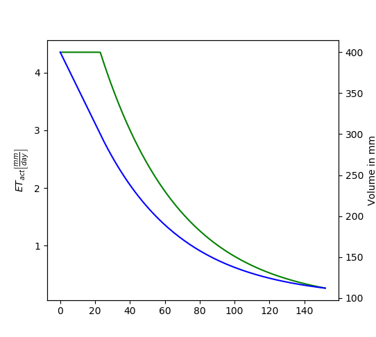
To put all of this long tutorial together in few lines of code, the task is to write a model that calculates the remaining volume in a lysimeter with a reference surface (short grass), with the following assumptions: