In this part, we are going to create a first model. To keep things simple, the model will be extremely simple. In fact, it would be easier to do this model in a spread sheet and keep cmf out of it. But of course it is to introduce some of the elements of cmf.

The model

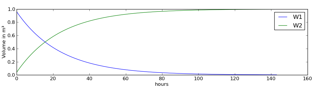
The model is a simple linear storage equation to transport water from one water storage ( \(W_1\)) to another water storage ( \(W_2\)).

\[ q_{W_1,W_2}=\frac{V_1}{t_r} \]

where:

\(q\) is the flux in \(\frac {m^3}{day}\) from \(W_1\) to \(W_2\)
\(V_1\) is the stored volume of water in \(W_1\) in \(m^3\)
\(t_r\) is the mean residence time of the water in \(W_1\) in days.

Implementation

The model (without the solver) is set up with the following lines of code:

import cmf
p = cmf.project()
# Create W1 in project p 
W1 = p.NewStorage(name="W1")
# Create W2 in project p without any volume as an initial state
W2 = p.NewStorage(name="W2")
# Create a linear storage equation from W1 to W2 with a residence time tr of one day
q = cmf.LinearStorageConnection(source=W1,target=W2,residencetime=1.0)
# Set the initial state of w1 to 1m³ of water.
W1.volume = 1.0

The ordinary differential equation (ODE) system

Formulation

With these lines the ODE (ordinary differential equation) system is formulated:

\[ \frac{dV_1}{dt} = -\frac{V_1}{t_r} \]

\[ \frac{dV_2}{dt} = \frac{V_1}{t_r} \]

Solving the system

Due to the simplicity of the model, it can be integrated analytically.

\[ V_1(t) = V_1(t_0) e^{-t/t_r} \]

\[ V_2(t) = V_1(t_0) (1-e^{-t/t_r}) \]

But it is of course only a proxy model. For more interesting models with stochastic boundary conditions, we need to use a numerical solution. For numerical time integration any of the time integration schemes of cmf will do for this model. If you are using more complex models with very different velocities, error controlled and implicit solvers are necessary.

Implementing the numerical solution

To integrate our simple system in time, we create an integrator, for example an explicit 4/5 step Runge-Kutta-Fehlberg integrator, the RKFIntegrator (other integrators are available, see later parts in the tutorial)

# Create an integrator (solver) for the ODE represented by project p, 
# with an error tolerance of 1e-9
solver = cmf.RKFIntegrator(p, 1e-9)
# Import Python's datetime module
import datetime
# Set the intitial time of the solver
solver.t = datetime.datetime(2012,1,1)

The code above is the setup part. Every cmf model consists of a setup part, where the hydrological system is defined. For larger models, Python's looping and conditional syntax and the possibility to read nearly any data format can help to define the system from data.

Running the system

Now we have all parts of our model available to run it. The solver can be advanced for a certain time step using solver.integrate(dt), where dt is a time step. After the integration the states and fluxes of the model can be queried (see Query fluxes and storages) and, if needed, saved into a file. Or you can store the results in a Python list or a cmf timeseries and use matplotlib to plot the results immediately after running the model. The content and format of output is completely up to the user, some experience in writing and reading files with Python is therefore a prerequisite to design your own output.

In this example, we will write a csv file with the timestep, the state of w1 and the state of w2.

# Create a csv file on disk for output, and write column headers
fout = open('firstmodel.csv','w')
fout.write('time,w1.volume m3,w2.volume m3\n')
# Run the model for 7 days, using a while loop
while solver.t < datetime.datetime(2012,1,7):
    # integrate the system for 1 h
    solver.integrate_until(solver.t + datetime.timedelta(hours=1))
    # write output (using the format operator %)
    fout.write('{t},{w1:0.4f},{w2:0.4f}\n'.format(t=solver.t,w1=W1.volume,w2=W2.volume))
fout.close()

In principle, this is the base for all cmf models. In the next chapters, we will introduce boundary conditions, more specialized water storages, like soil layers and rivers, and have a look at solute transport.

Alternative run time loop for plotting

An alternative way to the run time code above is using list comprehension. The result is then not written into a file, but stored in memory using a list. This list can be plotted using the pylab-API of matplotlib. The setup code is as before.

# Iterate the solver hourly through the time range and return for each time step the volume in W1 and W2
result = [[W1.volume,W2.volume] for t in solver.run(datetime.datetime(2012,1,1),datetime.datetime(2012,1,7),datetime.timedelta(hours=1))]
import pylab as plt
plt.plot(result)
plt.xlabel('hours')
plt.ylabel('Volume in $m^3$')
plt.legend(('W1','W2'))

And this is the result:

Next step is to include boundary conditions.