The first model from the last chapter is truely mass conservant. No water is entering or leaving the system. In this chapter the system will be opened up to be influenced by the system environment.

Creating an outlet

As a first step we will create a system outlet. The setup from the last chapter was:

# We are going to need the datetime module
import datetime
import cmf
p = cmf.project()
W1 = p.NewStorage(name="W1")
W2 = p.NewStorage(name="W2")
q = cmf.LinearStorageConnection(source=W1, target=W2, residencetime=1.0)
W1.volume = 1.0

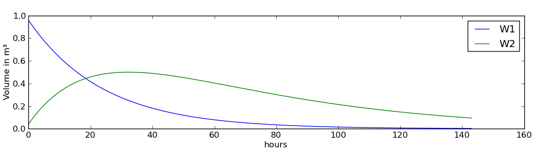
Now we add an outlet DirichletBoundary to the project and connect W2 with that outlet, using a linear storage connection with a longer residence time

Out = p.NewOutlet(name="Outlet")

qout = cmf.LinearStorageConnection(source=W2,target=Out,residencetime=2.0)

At last the new system needs to be solved again, the same way as the first model:

# Create the solver
solver = cmf.RKFIntegrator(p,1e-9)
# Iterate the solver hourly through the time range and return for each time step the volume in W1 and W2
result = [[W1.volume,W2.volume] for t in solver.run(datetime.datetime(2012,1,1),datetime.datetime(2012,1,7),datetime.timedelta(hours=1))]
import pylab as plt
plt.plot(result)
plt.xlabel('hours')
plt.ylabel('Volume in $m^3$')
plt.legend(('W1','W2'))
plt.show()

This results in:

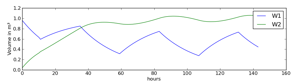
Creating an input boundary condition

To extend our model with input flux, we can add a Neumann boundary condition (NeumannBoundary) as a second boundary. This type of boundary condition is not triggered by the state of a water storage in the system, but by a defined flux given by the user. Since the flux should change over time, the flux is given as a timeseries. In this tutorial you will create a timeseries with daily alternating flux values between 0 and 1.

The setup code needs to be extended with the following:

# Create a Neumann Boundary condition connected to W1
In = cmf.NeumannBoundary.create(W1)
# Create a timeseries with daily alternating values.
In.flux = cmf.timeseries(begin = datetime.datetime(2012,1,1), 
                         step = datetime.timedelta(days=1), 
                         interpolationmethod = 0)
for i in range(10):
    # Add 0.0 m3/day for even days, and 1.0 m3/day for odd days
    In.flux.add(i % 2)

That's it. And the result is:

If the input timeseries is replaced by measured net rainfall data and the residence times of the storages are calibrated, you might be lucky to predict some catchments correctly. However, cmf contains many, many more connection types than linear storage connections. Some of the connection types are shown in the next chapters. A list of all connections is here.